Quick Start - Excel reports using ShufflePoint

ShufflePoint creates Excel reports by leveraging the built-in "Web Query" data import feature.
No Excel add-in is used, and you have the full capabilities of Excel at your disposal.

Key steps

1. Grant Access to a datasource
2. Download connection (IQY) file
3. Generate an access key
4. In Excel, create a web query

Key steps details

1. Grant Access. If you have not already done so, click Manage Datasources and then Google Analytics on the right side of the "My ShufflePoint" page, and follow instructions. Upon granting access, you will see a list of available accounts and profiles. You may also at this time select a default profile and timeframe.

   Setting up other datasources is done similarly. Some use OAuth while others use either an API key or credential.

2. Download an IQY file. Be sure to select "download file" instead of "open with Excel". Save the file in "My Documents/My Data Sources" in Windows or "/Applications/Microsoft Office 2011/Office/Queries" in MacOS.

   AQL IQY file
   BigQuery IQY file
   T-SQL IQY file

3. Get Key. Log into ShufflePoint, and click "Get Excel IQY files and keys" on the "My ShufflePoint" page. Select "Generate Un-scoped Key". Scoped vs. unscoped keys are explained on the key generator page. You can get a new key any time.

4. In Excel:

   1. Create a worksheet and paste into different cells:
      • The key generated above
      • A timeframe (eg. lastMonth)
      • Your Google Analytics profile id or name
      • Your AQL query
   2. Selected a destination cell, then
      Windows:
      • Click on Data > Get External Data > Existing Connections.
      • Select or browse for the IQY file you downloaded. Click Close.
      Mac:
      • Click on Data > Get External Data > Run Saved Query.
      • Select or browse for the IQY file you downloaded. Click Close.
      At first prompt, if not already selected, choose where you want the data to appear.
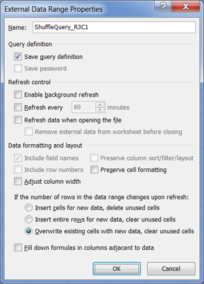
      Click "properties..." and in sub-prompt:

      • UNCHECK "Background refresh" (important to avoid "refresh all" errors)

      • UNCHECK "Adjust column width"

      • CHECK the third radio "Overwrite existing cells with new data, clear unused cells"

      Then at each of the following prompts, point to the cell that contains your key, timeframe, profile, and query.
      Check the boxes that say Use this value/refrence for future refreshes.

Notes

• If you split your query into multiple rows, then when selecting query cell, select ALL of the cells that contain your query.

• To run a different query, simply change the query in Excel. Likewise for timeframe or web profile.

• To run additional queries, follow all of the steps above and choose a different location where you want the data to appear.

• To refresh all queries, press Data > Refresh All.

• If your query is longer than 256 characters, Excel will not allow you to run the query (you may see a "bad parameter" message). There are two options for addressing this. First, you can spread your query across multiple adjacent rows. Or you can use our query shortener.

Example

Here are two sample queries you can paste into the query cell.

query 1: key metrics by browser

SELECT METRICS ga:uniquePageviews, ga:visits, ga:newVisits ON COLUMNS DIMENSIONS ga:browser ON ROWS TOP 10 BY ga:uniquePageviews DESC FROM default WHERE TIMEFRAME default

query 2: pageviews and bounce rate by continent

SELECT METRICS ga:pageviews, ga:bounceRate ON COLUMNS DIMENSIONS ga:continent ON ROWS BY ga:pageviews DESC FROM default WHERE TIMEFRAME default

If you use these two queries, and organize your IQY parameters the same, your resulting worksheet would look like:

Data Range Properties

The sub-prompt dialog should have these settings: